szlo statistics - A basic tutorial on plotting mixed effects using tidymodels

In R there are a ton of packages available to regression models including mixed effects model but one of the biggest issues is the vast difference in syntax needed for each of the modeling packages. Tidymodels was developed to solve this problem with the goal of having similar syntax style to the other tidyverse packages. Tidymodels itself is a “meta-package” consisting of a bunch {https://tidymodels.tidymodels.org/} of packages for modeling and statistical analysis with a focus on using the design philosophy of the tidyverse packages.

One of the current packages in development (as of this blog post) is the multilevelmod package for hierarchical modeling.

In this tutorial I am going to go through how to create a mixed effects model in R using the tidymodels and multilevelmod packages and how to plot the random intercepts using ggplot2. This blog post is just focused on using tidymodels and is not an indept overview of what mixed effects models are or how to use them.

First lets load our packages of interest. For the multilevelmod package (as of the time of this blog post) you will need to install it through github using devtools::install_github(). I ended up running into a little bit of a problem with an out of date Rcpp package. Deleting the folder manually and then re-installing ended up doig the trick. We will also be loading in one of R’s most used mixed effects modeling packages,lme4, to get some data.

#install.packages("pacman")
#load required packages
pacman::p_load("tidyverse","lme4")

# install multilevelmod
#devtools::install_github("tidymodels/multilevelmod")

library("multilevelmod")

Loading required package: parsnip

Now lets load in the sleep study dataset from the lme4 package. I am also going to create a fake categorical variable to use as a fixed effect in the model.

# load sleep study and create a fake category
set.seed(666) #\m/ rock on
sleepstudy <- lme4::sleepstudy %>% group_by(Subject) %>% 
              # creating a new random category with 3 levels to explore group effects
              mutate(cat = sample( LETTERS[1:3], 1, replace=TRUE, prob=c(0.25, 0.50, 0.25))) %>%
              ungroup()

The Tidymodels syntax requires that we set the “engine” for the type of model that we want to use. It is kind of like picking the type of car to use in MarioKart. You want to use the right engine for the right type of data. Since we are interested in looking at repeated measures data using a mixed effects model we will be using the “lmer” engine. We can set up the engine with the following code:

# set engine for mixed effects models
mixed_model_spec <- linear_reg() %>% set_engine("lmer")

Next we can build the model using Reaction as our dependent variable, Days and cat as our fixed effects and Subject as our random effect. The random effect syntax following that of the lme4 package using (1|Subject) to define Subject as the random intercept.

# create model
mixed_model_fit_tidy <- mixed_model_spec %>% fit(Reaction ~ Days + cat + (1 | Subject), data = sleepstudy)

mixed_model_fit_tidy

parsnip model object

Linear mixed model fit by REML ['lmerMod']
Formula: Reaction ~ Days + cat + (1 | Subject)
   Data: data
REML criterion at convergence: 1769.298
Random effects:
 Groups   Name        Std.Dev.
 Subject  (Intercept) 39.58   
 Residual             30.99   
Number of obs: 180, groups:  Subject, 18
Fixed Effects:
(Intercept)         Days         catB         catC  
    248.683       10.467        3.407       11.516

Now that we have created our model. Lets take a look at the predicted probabilities. To do this, we will create a data frame with all the different combinations of our fixed and random effects.

expanded_df_tidy <- with(sleepstudy,
                    data.frame(
                      expand.grid(Subject=levels(Subject),
                                  #cat = unique(cat),
                                  Days=seq(min(Days),max(Days),length=51))))

expanded_df_tidy <- sleepstudy %>% tidyr::expand(Subject,Days,cat)

expanded_df_tidy

# A tibble: 540 × 3
   Subject  Days cat  
   <fct>   <dbl> <chr>
 1 308         0 A    
 2 308         0 B    
 3 308         0 C    
 4 308         1 A    
 5 308         1 B    
 6 308         1 C    
 7 308         2 A    
 8 308         2 B    
 9 308         2 C    
10 308         3 A    
# … with 530 more rows

We can use this data frame and the predict() to get the predictions from our model.

predicted_df_tidy <- mutate(expanded_df_tidy,
                            pred = predict(mixed_model_fit_tidy,
                                           new_data=expanded_df_tidy, 
                                           type = "raw", opts=list(re.form=NA)))


predicted_df_tidy

# A tibble: 540 × 4
   Subject  Days cat    pred
   <fct>   <dbl> <chr> <dbl>
 1 308         0 A      249.
 2 308         0 B      252.
 3 308         0 C      260.
 4 308         1 A      259.
 5 308         1 B      263.
 6 308         1 C      271.
 7 308         2 A      270.
 8 308         2 B      273.
 9 308         2 C      281.
10 308         3 A      280.
# … with 530 more rows

When looking at the prediction output, notice that we are getting the same predictions for each subject. The predict function is currently giving us predictions for the fixed effects. If were were to run this same code using predict() with lme4 we would get the predictions for the random effects for each `Subject.

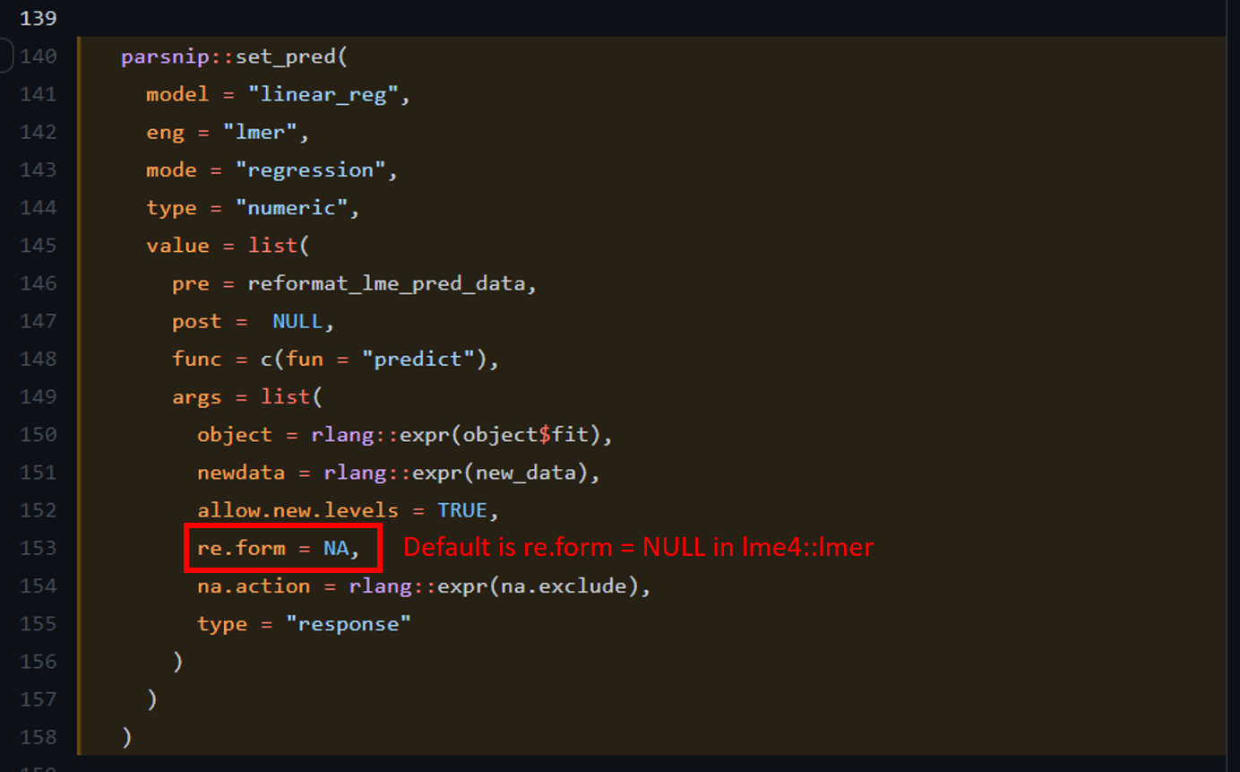
What is going on here? The issue is that multilevelmod package internally sets the default for prediction to re.form = NA;. In lme4 the default for predictions is re.form = NULL (i.e. include all random effects in the prediction).

knitr::include_graphics("tidymodel_git_comment.PNG")

We can include re.form = NULL in the predict() function by using the opts argument.

#update predictions
predicted_df_tidy <- mutate(expanded_df_tidy,
                            # get random predictions
                            pred_rand = predict(mixed_model_fit_tidy,
                                                new_data=expanded_df_tidy, 
                                                type = "raw", opts=list(re.form=NULL)),
                            # get fixed effect predictions
                            pred_fixed = predict(mixed_model_fit_tidy,
                                                new_data=expanded_df_tidy, 
                                                type = "raw", opts=list(re.form=NA)))

predicted_df_tidy

# A tibble: 540 × 5
   Subject  Days cat   pred_rand pred_fixed
   <fct>   <dbl> <chr>     <dbl>      <dbl>
 1 308         0 A          292.       249.
 2 308         0 B          296.       252.
 3 308         0 C          304.       260.
 4 308         1 A          303.       259.
 5 308         1 B          306.       263.
 6 308         1 C          314.       271.
 7 308         2 A          313.       270.
 8 308         2 B          317.       273.
 9 308         2 C          325.       281.
10 308         3 A          324.       280.
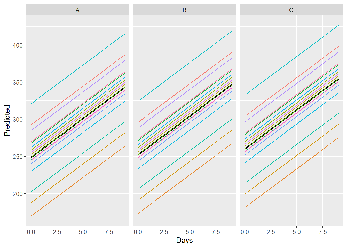
# … with 530 more rows

Now that we have both the predictions for the fixed and random effects we can plot them using ggplot2!

ggplot(predicted_df_tidy) +
       facet_wrap(.~cat) + 
       geom_line(aes(x=Days,y=pred_fixed), size = 1) + 
       geom_line(aes(x=Days,y=pred_rand,colour=Subject)) +
       scale_y_continuous("Predicted") + 
       theme(legend.position = "none")